A data science project can often be summarized a series of decisions. What do you do with missing data? What are you choosing as your target variable? Which kind of model are you choosing to make your predictions.
When I was working on my first machine learning classification project for the Flatiron School, the decision I probably spent the most time on was which metric to I should use to evaluate my models. There are various metrics one can use to check the performance of a classification model, and they generally deal with the number of true positives, true negatives, false positives, and false negatives.
When I was learning about them all, I was a bit overwhelmed by the math involved. It’s not the most complicated math you’ll come across as a data scientist, but I can’t count the number of times I conflated precision and recall because I couldn’t distinguish all the TPs, TNs, FPs, and FNs looked the same to me in the numerator and denominator. They’re not the easiest formulas to look at.
The math is important, but I ultimately had to understand them in plain English. So that’s what I’m going to attempt to lay out here: five important classification metrics in plain English. No math. No formulas.
Accuracy
This is probably the easiest metric to explain. Of all the samples, how many did your model label correctly? That’s it. It’s just the proportion of true positives and true negatives out of everything else. As with the rest of the metrics in this post, it can have a value between 0 and 1.
This seems like the most intuitive one to use, but it can easily be a victim to the class imbalance problem. If one class makes up 99% of the dataset, and your model learns to classify everything as that class, it will have 0.99 accuracy. Seems great, except the model will always get the minority class wrong. Not great.
Precision
Precision is the proportion of true positives out of all predicted positives. So the higher the number of false positives, the lower the precision score.
This is a useful metric when you need to optimize for a low amount of false positives (i.e. you don’t want to overcount the positive class). A common example is spam filters. It’s great if it’s only sending actual spam to your spam folder, but if it’s also classifying a lot of your important email as spam, then its precision score is probably low.
Recall
Recall is the flip side of precision. It’s the proportion of true positives out of actual positives. So it’s measuring how many positives your model got right. The higher the number of false negatives, the lower the recall score.
This is important when it’s costly to miss a positive case. The common example for this is medical situations where it’s better to be safe than sorry. If a model determines whether a patient is at risk (and should get tested) for a deadly disease, you don’t want it to incorrectly classify patients as not at risk. Therefore it would be important to be aware of the recall score.
F1
Let’s face it; this score is pretty much impossible to intuitively explain in plain English. F1 is the “harmonic mean” of precision and recall. It’s a formula that balances the precision and recall, since they tend to have an inverse relationship. This is useful in cases where you might be equally concerned about false positives and false negatives. F1 is often used in with datasets that have a class imbalance.
ROC-AUC
This is also often called AUROC or AUC. As with F1, it’s a bit of a doozy to understand without the math behind it. ROC stands for receiver operating characteristic, and it is a curve that shows the false positive rate and true positive rate at various probability thresholds. An example of one is show below.
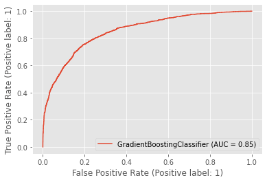
ROC-AUC is the area under this curve. It measures the ability of the model to assign a higher probability to a random positive sample higher than to a random negative sample. Another way of putting it: how well can the model distinguish between positive samples and negative samples? An AUC of 1 means it correctly labels all samples. An AUC of 0.5 means the model can’t distinguish between positive and negative samples at all.
These two blog posts do a good job of explaining ROC-AUC more in depth:
Classification metrics in scikit-learn
Once you understand the utility of all of these metrics, it’s important to know how to implement them. There are several ways to use do this is Python’s scikit-learn library.
- One way is to use the individual metric’s dedicated function in sklearn.metrics.
- Another way is to use sklearn.metrics.get_scorer and pass in the metric as a string corresponding to the metric.
The benefit of the latter way is that you don’t have to import each individual scorer function (sklearn.metrics.f1_score, sklearn.metrics.accuracy_score), as you may not know from the outset which metrics you’re going to use.
When running a grid search using GridSearchCV, you can also optimize for a specific metric using the “scoring” parameter.
